CARBON DIOXIDE BACKUP DATA REPORT (ID-172)
This report was revised June, 1990
Introduction
The evaluation of OSHA Method No. ID-172, Carbon Dioxide in Workplace Atmospheres (9.1.), was conducted when the time weighted average (TWA) Permissible Exposure Limit (PEL) for carbon dioxide (CO2) was 5000 ppm (1985). The PEL has been changed to 10,000 ppm TWA and a 30,000 ppm Short-Term Exposure Limit (STEL) has been added. Any mention of PEL in this report, unless specified otherwise, is in reference to the Transitional limit of 5,000 ppm. (Note: Some of the data in this report is presented as %CO2. To convert % to ppm, ppm CO2 = %CO2 x 10,000)
1. Experimental Protocol
1. The validation consists of the following experimental protocol:
2. Analysis of 3 sets of 6 spiked samples having concentration ranges of approximately 0.5, 1, and 2 times the PEL.
3. Analysis of 3 sets of 6 dynamically generated samples having concentration ranges of approximately 0.5, 1, and 2 times the PEL.
4. Determination of the qualitative and quantitative detection limit for analysis of CO2 by gas chromatography.
5. Determination of any variation in results when sampling at high and low humidity levels.
6. Comparison of other methods used for CO2 workplace determinations with the gas chromatographic method.
7. Determination of the storage stability of CO2 samples collected in gas sampling bags.
8. Assessment of the performance of the gas chromatographic method and conclusions.
Data for certain experiments were statistically examined for outliers and homogeneous variance. Possible outliers were determined using the American Society for Testing and Materials (ASTM) test for outliers (9.2.). Homogeneity of the coefficients of variation was determined using the Bartlett's test (9.3.).
2. Analysis
Procedure: Three sets of spiked samples were prepared and analyzed as follows:
2.1. Gas sampling bags were flushed with CO2-free compressed air [ambient CO2 and other potential contaminants were removed from the compressed air by using an air scrubber/filtration system (Figure 1) consisting mainly of a Ascarite II/Drierite bed]. A vacuum was then applied to completely evacuate the bags.
2.2. A known amount of CO2-free air was metered into each sampling bag. Compressed air flow rates were measured immediately before and after each experiment using a soap bubble flowmeter. Air flow was regulated by using a regulator-rotameter system as shown in Figure 1. Blank samples of the compressed air were periodically collected and analyzed along with the samples and standards.
2.3. A known amount of CO2 was metered into each sampling bag containing diluent air. Carbon dioxide flow rates for the spiked samples were determined immediately before and after each experiment using a soap bubble flowmeter. A gas cylinder containing 1.93% CO2 in air (Air Products, Long Beach, CA, certified analytical standard) was used for spiking the samples.
2.4. Reference and analytical standards were analyzed along with the spiked samples. The reference standard was purchased commerically (Scott Specialty Gases, Houston, TX, 0.9968% CO2 in nitrogen, methane, carbon monoxide, oxygen, and hydrogen, certified analytical standard) and analytical standards were generated by dilution of Bone Dry grade CO2 (Union Carbide, 99.8% min. purity). Carbon dioxide flow for analytical standards was regulated using a regulator-mass flow controller system as shown in Figure 2.
2.5. Spiked samples, blanks, reference, and generated standards were analyzed by gas chromatography (9.1.). Samples were analyzed within 2 days of preparation. Analytical instrument parameters are displayed in Appendix 1.
Results: Spiked sample results were calculated using a linear regression concentration-response curve. Integrated peak areas were used as signal measurement. Spiked sample recoveries are listed in Table 1. All Analysis data passed both the outlier and Bartlett's tests. The data (Table 1) indicates good precision and accuracy. The coefficient of variation for analysis (CV1) was 0.034 and the average analytical or spiked recovery was 95.2%.
3. Sampling and Analysis
Procedure: Three sets of generated samples were prepared and analyzed by:
3.1. Gas sampling bags were flushed with CO2-free compressed air. Ambient CO2 and other potential contaminants were removed from the compressed air by using an air filtration system similar to the one shown in Figure 1. A vacuum was then applied to completely evacuate the bags.
3.2. A dynamic gas generation system was assembled as shown in Figure 2. A humidity, temperature, and flow control system (Miller-Nelson Research Model 301) was used to control and monitor air flow. A dry test meter (Singer Co., Model # DTM 115) was to measure air flow immediately before, during, and after the experiments. The flow control system was calibrated in-house temperature, humidity, and flow prior to use. Calibration of the dry test meter was done using a spirometer as a primary standard.
3.3. Carbon dioxide (Bone Dry grade, 99.8% min. purity) gas was introduced into the flow system via a mixing chamber as shown in Figure 2. Carbon dioxide flow rates were taken immediately before and after each experiment using a soap bubble flowmeter. Flow rates were controlled using mass flow controllers (Tylan Model FC260 mass flow controller).
3.4. Generated samples, blanks, reference, and spiked standards were analyzed by gas chromatography. Reference standards were determined by direct injection of the gas from the canister into the gas sampling valve of the gas chromatograph. Analytical standards were prepared in gas sampling bags and then injected. Samples were analyzed within 2 days of preparation. Instrument parameters used during the analysis are displayed in Appendix 1.
Results: Generated sample results were calculated using a linear regression concentration response curve. Integrated peak areas were used as signal measurement. Generated sample recoveries are listed in Table 2. As shown in Table 2, the gas chromatographic determinations of CO2 using gas sampling bags are within NIOSH accuracy and precision guidelines (9.3.). The CVT was 0.026 and the overall recovery was 99.5%. The Sampling and Analysis data shows excellent precision and accuracy. All data passed both the outlier and Bartlett's test.
4. Detection Limit
Procedure: The qualitative detection limit for the analysis of CO2 by gas chromatography was calculated using the Rank Sum Test (9.4.). The International Union of Pure and Applied Chemistry (IUPAC) method for detection limit determinations was used to determine the quantitative limit (9.5.). The procedure used for sample preparation for determining the detection limit is shown below:
4.1. Same as Section 2.1.
4.2. Blank samples were generated using the flow, humidity, and temperature control system mentioned in Section 3.2.
4.3. Low concentration CO2 standards were prepared by mixing CO2 (1.93% in air), via a mixing chamber, with the treated air. Concentrations of 205.1, 398.9, and 662 ppm were used as standards.
4.4. Samples were then analyzed by gas chromatography. Analytical conditions used are given in Appendix 1.
Results: Qualitative and quantitative detection limits are listed in Tables 3 and 4, respectively. The qualitative limit is 200 ppm. The quantitative limit is 500 ppm. A 1-mL sampling loop was used for all analyses. Lower detection limits for CO2 are possible with larger sampling loops, but should not be necessary for workplace determinations. This assumption is based on the fact that ambient air will always contain a certain amount of CO2. In well ventilated areas, the level of CO2 is normally in the range of 300 to 700 ppm.
5. Humidity Study
Procedure: Samples were generated at high (80%), medium (50%), and low (25%) relative humidities using the same equipment and conditions described in Section 3. Samples were taken side-by-side with detector tube samples (9.6.).
Results: Gas sampling bag results at 80 and 25% RH are presented in Table 5. Table 2 contains the 50% RH test. Data from sampling at different humidities displayed no apparent effect on collection efficiency. As shown in Table 5, an analysis of variance (F test) was performed on the data to determine any significant difference among or within the different humidity groups. Variance at each concentration level (0.5, 1, and 2 times the PEL) was compared across the 3 humidity levels (25, 50, and 80% RH). The variance among and within the different concentration groups gave acceptable calculated F values with the exception of the test conducted at the PEL. Recovery at each humidity level was also considered. As also shown in Table 5, no evidence of any constant increase or decrease in average recovery is apparent across the humidity levels. The large calculated F value at the PEL was judged to be due to variation in sample generation and analysis and not to a humidity effect.
6. Comparison Methods
6.1. Detector tubes (in-house study)
A side-by-side (in-house) determination of CO2 was performed using different types of short-term CO2 detector tubes and simultaneous gas sampling bag-gas chromatography analysis. Detector tubes were chosen since they were listed as the OSHA sampling method for CO2 (9.8.). As mentioned in the Introduction of the CO2 method (9.1.), an alternative titration method (9.7.) was considered unsuitable to use for comparison at the generated concentration levels. Gas chromatographic and detector tube samples were taken at different humidity levels. A synopsis of the side-by-side testing is shown in Table 6. The overall recovery and CV for the gas sampling method displays an improvement over the detector tube technique. Further information regarding the short-term detector tube evaluation can be found in reference 9.6.
6.2. "Numbering error. This section contains no data."
6.3. A preliminary evaluation of long-term detector tubes was also performed (9.9.). The Draeger model no. 6728611 long-term detector tube and the Mine Safety Appliance Vaporgard Dosimeter were examined. Preliminary testing revealed the Draeger tube unsatisfactory for CO2 compliance determinations. Only 10 MSA dosimeters were tested and all were from the first lot of production. Dosimeter results were satisfactory; however, further testing and assessment of lot-to-lot variability are necessary.
6.4. Detector tubes (field study)
A side by side field sampling evaluation was also performed. The sampling was done at a food freezing plant which used liquid CO2 as the refrigerant. Gas bag samples and detector tubes were taken in various areas around the plant. Detector tubes were taken at random times and in close vicinity to the sampling bags. A log normal distribution was applied to the data to determine TWAs (for a further discussion of grab samples used to determine TWAs, see references 9.10. and 9.11.). Detector tube readings were also taken directly from the personal gas bag samples during the gas chromatographic analysis. Results of the field testing are also listed in Table 6.
6.5. Miran 1A
The Miran 1A infrared gas analyzer was also assessed for possible use in CO2 determinations. As a direct reading instrument, the Miran 1A appeared too sensitive to assess large CO2 levels sometimes found in industrial settings. An off-scale reading was given when CO2 concentrations were above 5,000 ppm. However, this response characteristic of the MIRAN appears to make it useful for indoor air quality investigations because CO2 levels less than 5,000 ppm are normally used to determine ventilation system performance. Carbon dioxide is also used in air quality assessments as a tracer gas to monitor ventilation efficiency.
An attempt was also made to use the 5.4-L sampling cell of the gas analyzer as a closed-system analyzer. Samples were collected in gas sampling bags and aliquots were taken from the bags using gas-tight syringes. These aliquots were then injected into the closed system. It was necessary to take 50 to 100-mL aliquots to achieve an adequate signal for CO2 measurement at the generated levels. The aliquots were considered very large and made accurate and precise analysis difficult.
7. Stability Test
Procedure: A long-term evaluation of sample media stability was performed to determine any potential problems if delays in sample analyses occur. Five layered, 5-L sampling bags containing generated samples, field samples, and reference standards were used to assess CO2 storage stability. Samples were analyzed at various times, up to 50 days, after sample collection. A few samples were stored in a refrigerator at 5 °C and analyzed periodically over 31 days. Recovery data are listed in Table 7 and graphically represented in Figure 3.
Results:
Note: Previously, different types of gas sampling bags were evaluated for stability, structural integrity, and compactness. Tedlar sampling bags can be used for standard dilution, provided the standards are analyzed within a 24-h period. A significant loss of CO2 was noted if Tedlar bag standards were analyzed during longer periods.
The storage ability of the five-layered, 5-L gas sampling bag for
CO2 is unacceptable if stored for a period longer than 14
days. Table 7 individually lists each sample/result. A summary of the
stability data per time period is listed below:
| Total Samples | Day | Ave % Recovery |
| 10 | 1-5 | 95.6 |
| 8 | 9-18 | 89.7 |
| 8 | 26-31 | 77.2 |
| 7 | >31 | 68.5 |
Figure 3 graphically depicts the recovery dropping below 90% after 14 days of storage. Sample refrigeration appears to slightly retard CO2 loss; however, gas bag samples should be sent to the laboratory and analyzed as soon as possible.
8. Method Performance - Conclusions
The data generated during the validation of the method indicate an acceptable alternative for sampling and analyzing CO2. The gas chromatographic method offers an accurate and precise assessment of CO2 exposures in the workplace. Although no samples were taken at concentration levels at the 30,000 ppm STEL, the storage stability data at about 20,000 ppm indicates the stability, precision, and accuracy were similar to validation range (2,000 to 10,000 ppm) results. Standards prepared at 30,000 ppm to determine the linear working range displayed excellent linearity with lower concentration standards used to construct the concentration-response curve.
This method should be capable of accurate and precise measurements to determine compliance with the 10,000 ppm PEL and also the 30,000 ppm STEL.
9. References
9.1. Occupational Safety and Health Administration Technical Center: Carbon Dioxide in Workplace Atmospheres (OSHA-SLTC Method No. ID-172). Salt Lake City, UT. Revised 1990.
9.2. Mandel, J.: Accuracy and Precision, Evaluation and Interpretation of Analytical Results, The Treatment of Outliers. In Treatise On Analytical Chemistry, 2nd ed., Vol. 1, edited by I.M. Kolthoff and P.J. Elving. New York, NY: John Wiley and Sons, 1978. pp. 282-285.
9.3. National Institute for Occupational Safety and Health: Documentation of the NIOSH Validation Tests by D. Taylor, R. Kupel and J. Bryant (DHEW/NIOSH Pub. No. 77-185). Cincinnati, OH: National Institute for Occupational Safety and Health, 1977. pp. 1-12.
9.4. National Bureau of Standards: Experimental Statistics by M.G. Natrella (NBS Handbook 91). Washington, DC: U.S. Department of Commerce, National Bureau of Standards, 1966. Chapter 16, pp. 8-14.
9.5. Long, G.L. and J.D. Winefordner: Limit of Detection -- A Closer Look at the IUPAC Definition. Anal. Chem. 55: 712A-724A (1983).
9.6. Occupational Safety and Health Administration Analytical Laboratory: Carbon Dioxide Detector Tubes (PE-2). Salt Lake City, UT. 1987.
9.7. Norton, J. F., ed.: Standard Methods for the Examination of Water and Sewage. 9th ed. New York, NY: American Public Health Association, 1946. pp. 33-40.
9.8. U.S. Department of Labor-Occupational Safety and Health Administration: Chemical Information File. Online Database -- OSHA Information System. Washington, DC: Directorate of Technical Support, U.S. Dept. of Labor, OSHA, 1985.
9.9. Occupational Safety and Health Administration Analytical Laboratory: Carbon Dioxide Detector Tubes -- Long Term (PE-3). Salt Lake City, UT. 1987.
9.10. National Institute for Occupational Safety and Health: Occupational Exposure Sampling Strategy Manual by N.A. Leidel, K.A. Busch and J.R. Lynch (DHEW/NIOSH Pub. No. 77-173). Washington, DC: Government Printing Office, 1977.
9.11. Leichnitz, K.: Detector Tube Measuring Techniques. Ecomed, Federal Republic of Germany, 1983. pp. 251-264.
Table 1
Analysis
|
| |||||||
| Level | %CO2 Taken | %CO2 Found | F/T | n | Mean | Std Dev | CV1 |
|
| |||||||
| 0.251 | 0.248 | 0.986 | |||||
| 0.251 | 0.234 | 0.931 | |||||
| 0.5 X PEL | 0.251 | 0.236 | 0.939 | ||||
| 0.251 | 0.236 | 0.939 | |||||
| 0.251 | 0.239 | 0.951 | |||||
| 0.251 | 0.236 | 0.939 | |||||
| 6 | 0.947 | 0.020 | 0.021 | ||||
| 0.497 | 0.505 | 1.016 | |||||
| 0.497 | 0.470 | 0.946 | |||||
| 1 X PEL | 0.497 | 0.467 | 0.940 | ||||
| 0.497 | 0.452 | 0.909 | |||||
| 0.497 | 0.477 | 0.960 | |||||
| 0.497 | 0.452 | 0.909 | |||||
| 6 | 0.947 | 0.040 | 0.042 | ||||
| 1.007 | 1.008 | 1.001 | |||||
| 1.007 | 0.964 | 0.957 | |||||
| 2 X PEL | 1.007 | 0.995 | 0.988 | ||||
| 1.007 | 0.984 | 0.977 | |||||
| 1.007 | 0.953 | 0.946 | |||||
| 1.007 | 0.911 | 0.904 | |||||
| 6 | 0.962 | 0.035 | 0.036 | ||||
F/T = Found/Taken
CV1(Pooled) = 0.034
Average Recovery = 0.952
Table 2
Sampling and Analysis (50% RH, 25 °C)
|
| ||||||||
| Level | %CO2 Taken | %CO2 Found | F/T | Airvol | n | Mean | Std Dev | CV2 |
|
| ||||||||
| 0.270 | 0.270 | 0.998 | 1.7 | |||||
| 0.270 | 0.266 | 0.983 | 2.1 | |||||
| 0.5 X PEL | 0.270 | 0.269 | 0.994 | 2.7 | ||||
| 0.270 | 0.275 | 1.016 | 3.5 | |||||
| 0.270 | 0.274 | 1.013 | 3.9 | |||||
| 0.270 | 0.269 | 0.994 | 2.5 | |||||
| 6 | 1.000 | 0.013 | 0.013 | |||||
| 0.544 | 0.563 | 1.036 | 3.6 | |||||
| 0.544 | 0.560 | 1.030 | 3.4 | |||||
| 1 X PEL | 0.544 | 0.565 | 1.039 | 3.1 | ||||
| 0.544 | 0.560 | 1.030 | 1.7 | |||||
| 0.544 | 0.546 | 1.004 | 2.1 | |||||
| 0.544 | 0.556 | 1.023 | 4.1 | |||||
| 6 | 1.027 | 0.013 | 0.012 | |||||
| 1.005 | 0.981 | 0.976 | 3.0 | |||||
| 1.005 | 0.935 | 0.930 | 3.1 | |||||
| 2 X PEL | 1.005 | 0.975 | 0.970 | 1.6 | ||||
| 1.005 | 0.969 | 0.964 | 3.2 | |||||
| 1.005 | 0.961 | 0.956 | 3.2 | |||||
| 1.005 | 0.952 | 0.947 | 4.1 | |||||
| 6 | 0.957 | 0.017 | 0.018 | |||||
| Airvol | = | Air volume taken (L) |
| F/T | = | Found/Taken |
| CV2(Pooled)/FONT> | = | 0.014 |
| CVT | = | 0.026 |
| Bias | = | -0.005 |
| Overall Error | = | ±5.7% |
Table 3
Determination of Qualitative Detection Limit
| ppm | Integrated Area | |
|
|
| |
| BLANK | 0, 0, 0, 0, 0, 0, 0, 0, 130, 275 | |
| 205.1 | 221, 242, 314, 324, 426, 504, 548, 563 | |
| 398.9 | 967, 1041, 1075, 1249, 1267, 1268, 1334, 1421 | |
| 662 | 2090, 2107, 2335, 2561 |
Rank Sum Data
| a | = | 0.01 (two-tailed test) |
| n1 | = | 8 (# of 205.1 ppm determinations) |
| n2 | = | 10 (# of blank determinations) |
| n | = | n1 + n2 = 18 |
| R | = | 114 (sum of ranks for 205.1 ppm) |
| Rn | = | n1(n+1) - R = 38 |
| R(table) | = | 47 |
Therefore, Rn is not equal to or greater than R(table), and both sample populations are significantly different.
Qualitative detection limit = 205.1 ppm
Table 4
Determination of Quantitative Detection Limit
IUPAC Method
| Using the equation: | Cld = k(sd)/m |
Where:
| Cld | = | the smallest detectable concentration an analytical instrument can determine at a given confidence level. |
| k | = | 3, thus giving 99.86% confidence that any detectable signal will be greater than or equal to an average blank reading plus three times the standard deviation (area reading > Blave + 3sd). |
| sd | = | standard deviation of blank readings. |
| m | = | analytical sensitivity or slope as calculated by linear regression. |
Minimum detectable signal:
| Cld = 3(91.97/1.771) | |
| Cld = 156 ppm |
For k = 10 (Quantitative detection limit, 99.9% Confidence):
| Cld = 519 ppm as a reliable detectable signal |
Table 5
Humidity Tests
25% RH (25 °C)
|
| |||||||
| Level | %CO2 Taken | %CO2 Found | F/T | n | Mean | Std Dev | CV |
|
| |||||||
| 0.266 | 0.293 | 1.100 | |||||
| 0.266 | 0.277 | 1.040 | |||||
| 0.5 X PEL | 0.266 | 0.266 | 1.000 | ||||
| 0.266 | 0.282 | 1.060 | |||||
| 0.266 | 0.282 | 1.060 | |||||
| 5 | 1.052 | 0.036 | 0.035 | ||||
| 0.538 | 0.483 | 0.898 | |||||
| 0.538 | 0.506 | 0.941 | |||||
| 1 X PEL | 0.538 | 0.509 | 0.947 | ||||
| 0.538 | 0.499 | 0.929 | |||||
| 4 | 0.929 | 0.022 | 0.023 | ||||
| 1.002 | 1.001 | 0.999 | |||||
| 1.002 | 1.012 | 1.010 | |||||
| 2 X PEL | 1.002 | 0.957 | 0.955 | ||||
| 1.002 | 0.982 | 0.980 | |||||
| 1.002 | 0.995 | 0.993 | |||||
| 5 | 0.987 | 0.020 | 0.021 | ||||
F/T = Found/Taken
CV(Pooled) = 0.027
Average Recovery = 0.989
Table 5 (Cont.)
Humidity Tests
80% RH (25 °C)
|
| |||||||
| Level | %CO2 Taken | %CO2 Found | F/T | n | Mean | Std Dev | CV |
|
| |||||||
| 0.268 | 0.300 | 1.120 | |||||
| 0.268 | 0.289 | 1.080 | |||||
| 0.5 X PEL | 0.268 | 0.281 | 1.050 | ||||
| 0.268 | 0.276 | 1.030 | |||||
| 0.268 | 0.270 | 1.010 | |||||
| 5 | 1.058 | 0.043 | 0.041 | ||||
| 0.530 | 0.493 | 0.930 | |||||
| 0.530 | 0.484 | 0.912 | |||||
| 1 X PEL | 0.530 | 0.498 | 0.939 | ||||
| 0.530 | 0.483 | 0.910 | |||||
| 0.530 | 0.490 | 0.923 | |||||
| 5 | 0.923 | 0.012 | 0.013 | ||||
| 1.002 | 0.952 | 0.950 | |||||
| 1.002 | 0.908 | 0.906 | |||||
| 2 X PEL | 1.002 | 0.970 | 0.968 | ||||
| 1.002 | 0.985 | 0.983 | |||||
| 1.002 | 0.954 | 0.952 | |||||
| 5 | 0.952 | 0.030 | 0.030 | ||||
| F/T = Found/Taken | |||||||
| CV(Pooled) = 0.030 | Average Recovery = 0.978 | ||||||
|
| |||||||
| F Test Results | Recoveries % | |||||||
|
|
| |||||||
| Level | F(calc) | F(0.99) | df | 25% | 50% | 80% | RH | |
| 0.5 X PEL | 5.55 | 6.70 | 2,13 | 105.2 | 100.0 | 105.8 | ||
| 1 X PEL | 79.4* | 6.93 | 2,12 | 92.9 | 102.7 | 92.3 | ||
| 2 X PEL | 3.73 | 6.70 | 2,13 | 98.7 | 95.7 | 95.2 | ||
| Average | 98.9 | 99.5 | 97.8 | |||||
df = degrees of freedom
* Large F value appears to be due to variability in sample generation and not to any humidity effect.
Table 6
Comparison of Detector Tube and Gas Chromatograph Analyses
| In-house Samples - Side-by-Side | ||||||
|
| ||||||
| Detector Tube Recoveries | Gas Chromatograph | Recoveries | ||||
| Tube Mfg. | N | Recovery% | Pooled CV | N | Recovery | Pooled CV |
|
| ||||||
| MSA (50% RH) | 9 | 111.8 | 0.069 | 5 | 107.9 | 0.012 |
| Kitagawa (50% RH) | 9 | 108.0 | 0.039 | 8 | 103.0 | 0.050 |
| Gastec (25% RH) | 18 | 101.3 | 0.063 | 11 | 98.8 | 0.031 |
| Gastec (50% RH) | 17 | 109.9 | 0.058 | 7 | 106.5 | 0.014 |
| Gastec (80% RH) | 18 | 106.2 | 0.057 | 13 | 97.8 | 0.032 |
| Draeger (50% RH) | 9 | 101.8 | 0.076 | 6 | 100.2 | 0.010 |
| Totals | 80 | 106.5 | 0.039-0.076 | 50 | 102.3 | 0.01-0.050 |
|
| ||||||
Detector Tube - Gas Chromatography Statistical Summary
| Detector Tube Pooled CV2 (all tubes) | = | 0.025-0.076 |
| Ave. Recovery, Detector Tubes (all tubes) | = | 85.9-111.8% |
| Gas Chromatograph (CV2 Pooled) | = | 0.014 |
| Gas Chromatograph (CVT Pooled) | = | 0.026 |
| Average Recovery, GC | = | 99.5% |
| Average Recovery, GC (all samples) | = | 95-103% |
| Field Samples | ||||||
|
| ||||||
| Sample # | Detector Tube Recoveries | GC Recoveries | ||||
| Type | N | AV R% | LAV R% | Bagtube | ppm CO2 | |
|
| ||||||
| 1A | P | 7 | 76 | 73 | 104% | 11,000 |
| 1B | P | 7 | 81 | 77 | 93% | 15,000 |
| 2A | P | 6 | 83 | 80 | 86% | 8,000 |
| 2B | P | 7 | 83 | 74 | 83% | 7,600 |
| 3A | A | 5 | 84 | 83 | -- | 8,900 |
| 3B | A | 6 | (11000) | (9100) | -- | LIS* |
| 4A | A | 3 | 97 | 96 | -- | 6,800 |
| 4B | A | 6 | 72 | 62 | -- | 5,300 |
| 5A | A | 4 | 92 | 89 | -- | 7,200 |
| 5B | A | 5 | 92 | 84 | -- | 9,700 |
| N | = | Number of tubes or samples taken |
| *LIS | = | Lost in shipment. Tube results for this sample are, listed in ppm. |
| AV R% | = | Average recovery in %, normalized to GC results. |
| LAV R% | = | Log normal average results in %, also normalized (9.10., 9.11.). |
| Bagtube | = | Detector tube sample taken on gas sampling bag prior to gas chromatographic analysis. Bagtube samples were only taken from the personal samples. |
| P | = | Personal sample |
| A | = | Area sample |
Table 7
Stability Test (Per Sample)
|
| |||
| ppm Taken | ppm Found | Recovery % | Day |
|
| |||
| 5260 | 5150 | 97.9 | 5 |
| " " | 4760 | 90.5 | 18 |
| " " | 3980 | 75.7 | 29 |
| " " | 3650 | 68.9 | 50+ |
| 5440 | 4670 | 85.9 | 11* |
| " " | 4370 | 80.4 | 31+ |
| " " | 4840 | 89.1 | 11* |
| " " | 4720 | 86.9 | 31*+ |
| " " | ="2">4990 | 91.8 | 11* |
| " " | 5010 | 92.1 | 31*+ |
| 6770 | 6550 | 96.8 | 5 |
| 7210 | 7020 | t face="Arial" size="2">97.4 | 5 |
| 7570 | 7140 | 94.3 | 5 |
| " " | 6880 | 90.9 | 18 |
| " " | 6060 | 80.1 | 29 |
| " " | 5730 | 75.7 | 50+ |
| 7990 | 7170 | 89.7 | 5 |
| " " | 6210 | 77.7 | 18 |
| " " | 5010 | 62.7 | 29 |
| " " | 4490 | 56.2 | 50+ |
| 8940 | 8280 | 92.6 | 5 |
| " " | 7810 | 87.4 | 18 |
| " " | 6380 | 71.4 | 29 |
| " " | 5040 | 56.4 | 50+ |
| 11010 | 10420 | 94.6 | 5 |
| " " | 10750 | 97.6 | 18 |
| " " | 9550 | 86.7 | 29 |
| " " | 8850 | 80.4 | 50+ |
| 14600 | 14240 | 97.5 | 5 |
| " " | 13940 | 95.5 | 18 |
| " " | 12900 | 88.3 | 29 |
| " " | 12040 | 82.5 | 50+ |
| 19300 | 19280 | 99.9 | 2 |
| " " | 18410 | 95.4 | 5 |
| " " | 17930 | 92.9 | 9 |
| " " | 16460 | 85.3 | 14 |
| " " | 13990 | 72.5 | 26 |
| " " | 11330 | 58.7 | 37 |
* Samples stored in refrigerator at 5 °C. Data for refrigerated samples
is not included in final calculations. All other samples were stored at 20
°C.
+ All samples were analyzed using a 1 mL gas sampling loop, with
the exception of the (+) day stability study. On that day, a 5 mL loop was
used.
Appendix 1
Analysis Parameters for CO2 Determinations
Gas chromatograph (Hewlett-Packard 5730a gas chromatograph)
| Detector | Thermal conductivity |
| Sensitivity | 5 |
| Helium flow rate | 15 - 25 mL/min |
| Column temperature | ambient (20 to 25 °C) |
| Detector temperature | ambient (20 to 25 °C) |
| Valve manifold temperature | ambient (20 to 25 °C) |
| Column | Chromosorb 102 (6 ft X 1/4 in. stainless steel, 80/100 mesh) |
| Gas sampling loop | 1 mL |
Integrator (Hewlett-Packard 3385a automation system)
| Attenuation | 4 |
| Run time | 3.5 min |
| Peak time | 2.6 - 2.9 min |
| External valve switch | 0.01 s (from start of integration to valve opening) |
| Auxiliary signal | a |
| Chart speed | 1 |
| Zero | 10 |
| Area reject | 0 |
Generation of Dilution Air (CO2-free)
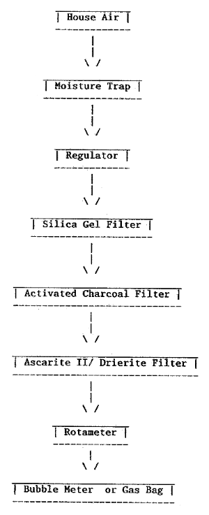
Figure 1
Carbon Dioxide - Air Flow
Generation System
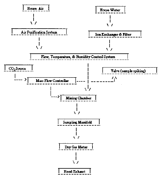
Figure 2
Storage Stability - Carbon
Dioxide in Gas Sampling Bags
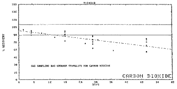
Figure 3