| Method no.: | 100 |
| Matrix: | Air |
| Target concentration: | 1000 ppm (1900 mg/m3) |
| Procedure: | Samples are collected by drawing air through two
|
| Recommended air volume and sampling rate: |
12 L at 0.05 L/min |
| Reliable quantitation limit: | 0.68 ppm (1.29 mg/m3) |
| Standard error of estimate at the target concentration: |
5.17% |
| Special requirement: | The air sampler must be separated into its component sampling
tubes as soon as possible after sampling. This will prevent
|
| Status of method: | Evaluated method. This method has been subjected to the established evaluation procedures of the Organic Methods Evaluation Branch. |
| Date: April 1993 | Chemist: Warren Hendricks |
Organic Methods Evaluation Branch
OSHA Salt
Lake Technical Center
Salt Lake City, UT 84165-0200
1. General Discussion
1.1. Background
1.1.1. History
Previous to this method, OSHA had been using a procedure based on
NIOSH Method 1400 (Ref.
5.1.) to collect and analyze ethyl alcohol samples. Method 1400
requires sample collection on
A post-sampling migration test for ethyl alcohol was performed using samples collected on the sampling medium recommended in Method 1400. These samples were collected for 20 min at 0.05 L/min from a test atmosphere containing 980 ppm of ethyl alcohol at 78% relative humidity and 26°C. Eighteen percent of the collected ethyl alcohol migrated into the sampling tube back section during two weeks of ambient storage. Much less migration (0.3%) was observed in similar samples stored at 5°C. The shipping restrictions of Method 1400 are inconvenient, but do help alleviate a serious migration problem.
The purpose of this work was to develop a collection method which
permitted ambient temperature sample shipment, and which also
utilized a sampler with more capacity for ethyl alcohol than the
charcoal sampler in Method 1400. The use of Anasorb 747 to collect
methyl alcohol vapors was reported in OSHA Method
91 (Ref.
5.2.). Sampler capacity tests showed that Anasorb 747 had ample
capacity for ethyl alcohol, however, ethyl alcohol (like methyl
alcohol) was found to undergo
This method features sample collection on Anasorb 747, desorption
with 60/40
Anasorb 747 is a proprietary beaded active carbon marketed by
SKC, Inc. It is reported to have a low ash content, a surface more
hydrophobic and catalytically less active than
1.1.2. Toxic effects (This section is for information only and should not be taken as the basis of OSHA policy.)
The lethal dose for ethyl alcohol administered by inhalation to rats is about 13,000 ppm after 22 h; to guinea pigs, about 22,000 ppm after 9 h; and to mice, about 29,000 ppm after 7 h (Ref. 5.4.).
The OSHA PEL for ethyl alcohol is 1000 ppm based on an 8-h TWA (Ref. 5.5.). The minimum concentration of ethyl alcohol that can be identified by odor has been reported to be 350 ppm. Exposure to concentrations of 5,000 to 10,000 ppm ethyl alcohol can result in irritation of the eyes and of the upper respiratory tract mucous membranes. Concentrations of this level have an intense odor, but most people become acclimated after a short time. If exposure at these levels continues, the result can be stupor or drowsiness. An air concentration of 15,960 ppm, which could be tolerated only with discomfort, caused continuous lacrimation and marked coughing. An air concentration of 21,280 ppm was described as intolerable, even for short periods. There is disagreement among experts on whether inhalation of ethyl alcohol vapors can cause drunkenness. (Ref. 5.6.) Splashes of the liquid in the eyes cause immediate stinging and burning, with reflex closing of the lids and tearing, transitory injury of the cornea, and hyperemia of the conjunctiva (Ref. 5.4.). Direct skin contact with the liquid may cause mild redness and burning. Skin sensitization has been reported. Prolonged or repeated contact with the liquid can cause dermatitis and defatting of the skin (Ref. 5.7.).
International Agency for Research on Cancer (IARC), in a monograph that did not consider occupational exposure to ethyl alcohol or exposure other than by drinking, concluded that alcoholic beverages are carcinogenic to humans. IARC further concluded that there is inadequate evidence for the carcinogenicity of ethyl alcohol and of alcoholic beverages in experimental animals. IARC made a distinction between alcoholic beverages and ethyl alcohol. Alcoholic beverages contain many constituents other than ethyl alcohol and water. (Ref. 5.8.)
1.1.3. Workplace exposure
Ethyl alcohol can be produced by direct catalytic hydration (or with ethyl sulfate as an intermediate) from ethylene, by fermentation of biomass, and by enzymatic hydrolysis of cellulose (Ref. 5.9.).
Several administrative and chemical controls have been
implemented to avoid taxation of ethyl alcohol. The administrative
controls include bonds, permits and scrupulous recordkeeping.
Chemical controls involve the use of denaturants that make the ethyl
alcohol unsuitable for beverage use. Some of the denatured ethyl
alcohols that may be encountered in the workplace include: denatured
ethyl alcohol (unpalatable for beverages), completely denatured
ethyl alcohol (unfit for beverages), specially denatured alcohol
(unfit for beverages but useful for specific applications), and
proprietary solvents and special industrial solvents. (Ref.
5.6.) Some of the many chemicals that are used to denature ethyl
alcohol include: methyl alcohol, brucine, brucine sulfate, quassin,
Ethyl alcohol is used in the manufacture of acetaldehyde, acetic
acid, ethylene, butadiene,
The total U.S. industrial production of ethyl alcohol in 1975 was 264 million gallons (Ref. 5.6.). The U.S. capacity for fuel ethyl alcohol was reported to be more than 1 billion gallons in 1992 (Ref. 5.11.).
No estimate of the number of workers potentially exposed to ethyl alcohol was found.
1.1.4. Physical properties and other descriptive information (Ref.
5.7.)
| chemical name: | ethyl alcohol |
| CAS no.: | 64-17-5 |
| molecular wt: | 46.07 |
| boiling point: | 78°C |
| melting point: | -117°C |
| specific gravity: | 0.7893 |
| vapor pressure: | 40 mmHg at 19°C (5 kPa) |
| vapor density: | 1.59 |
| evaporation rate: | 1.4 (carbon tetrachloride = 1) |
| flash point: | 55°F |
| explosive limits: | upper, 19%; lower, 3.3% |
| description: | a clear, colorless, volatile liquid with a pleasant odor, and a burning taste |
| solubility: | soluble in water, benzene, ether, acetone, chloroform, methyl alcohol, and many other organic solvents |
| synonyms: | ethanol; ethyl alcohol, 100%; alcohol; alcohol anhydrous;
Algrain; Anhydrol; ethyl hydrate; ethyl hydroxide; Jaysol;
Tecsol; |
| structural formula: | CH3CH2OH |
The analyte air concentrations throughout this method are based on
the recommended sampling and analytical parameters. Air concentrations
listed in ppm and ppb are referenced to 25°C and 101.3 kPa (760
mmHg).
1.2. Limit defining parameters
1.2.1. Detection limit of the analytical procedure
The detection limit of the analytical procedure is 40 pg per injection. This is the amount of analyte that will produce a peak with a height that is approximately 5 times the baseline noise. (Section 4.1.)
1.2.2. Detection limit of the overall procedure
The detection limit of the overall procedure is 15.52 µg per sample. This is the amount of analyte spiked on the sampling device that, upon analysis, produces a peak similar in size to that of the detection limit of the analytical procedure. This detection limit corresponds to an air concentration of 0.68 ppm (1.29 mg/m3). (Section 4.2.)
1.2.3. Reliable quantitation limit
The reliable quantitation limit is 15.52 µg per sample.
This is the smallest amount of analyte which can be quantitated
within the requirements of a recovery of at least 75% and a
precision (±1.96 SD) of ±25% or better. This reliable quantitation
limit corresponds to an air concentration of 0.68 ppm (1.29
mg/m3). (Section
4.3.)
The reliable quantitation limit and detection limits reported in
the method are based upon optimization of the instrument for the
smallest possible amount of analyte. When the target concentration
of analyte is exceptionally higher than these limits, they may not
be attainable at the routine operating parameters.
1.2.4. Instrument response to the analyte
The instrument response over concentration ranges representing 0.5 to 2 times the target concentration was linear. (Section 4.4.)
1.2.5. Recovery
The recovery of ethyl alcohol from samples used in the 16-day ambient storage test remained above 102%. (Section 4.5., regression line of Figure 4.5.1.)
1.2.6. Precision (analytical procedure)
The pooled coefficient of variation obtained from replicate determinations of analytical standards at 0.5, 1 and 2 times the target concentration is 0.014. (Section 4.6.)
1.2.7. Precision (overall procedure)
The precision at the 95% confidence level for the 16-day ambient temperature storage test is ±5.17%. (Section 4.7.) This includes an additional ±5% for sampling error.
1.2.8. Reproducibility
Six samples, collected from a controlled test atmosphere, and a draft copy of this procedure were submitted to SLTC for analysis. The samples were analyzed after 5 days of storage at about 5°C. No individual sample result deviated from its theoretical value by more than the precision reported in Section 1.2.7. (Section 4.8.)
2. Sampling Procedure
2.1. Apparatus
2.1.1. A personal sampling pump that can be calibrated within ±5% of the recommended flow rate with the sampling device in line.
2.1.2. A sample is collected using a 400-mg and a 200-mg Anasorb
747 sampling tube. The sampling tubes
2.2. Reagents
No reagents are required for sampling.
2.3. Technique
2.3.1. Break off both ends of the sampling tubes immediately
before sampling. The holes in the broken ends of the sampling tubes
should be approximately 1/2 the i.d. of the sampling tube. All tubes
should be from the same lot. Connect the outlet end of a
2.3.2. Connect the sampling tube to the sampling pump with
flexible tubing so that the sampled air passes through the inlet end
of the
2.3.3. Sampled air should not pass through any hose or tubing before entering the front sampling tube.
2.3.4. Attach the sampler vertically in the worker's breathing
zone, with the
2.3.5. Remove the sampling device after sampling for the
appropriate time. Separate the two sampling tubes and seal the tube
ends with plastic end caps. Wrap each sample
2.3.6. Submit at least one blank with each set of samples. The blank should be handled the same as the other samples except no air is drawn through it.
2.3.7. Record the sample air volume (in liters of air) for each sample. Note any potential interferences, such as chemicals used to denature the ethyl alcohol.
2.3.8. Ship any bulk sample separate from air samples.
2.4. Sampler capacity
Sampler capacity studies (Section 4.9.) were performed using controlled test atmospheres and 400-mg front sampling tubes. The average ethyl alcohol concentration of these test atmospheres was 3640 mg/m3 (1932 ppm) at 85% relative humidity and 25°C. The sampling rate was 0.05 L/min. The average 5% breakthrough air volume was 15.2 L. Five percent breakthrough was defined as the point at which the effluent from the sampling tube contained ethyl alcohol at a concentration equivalent to 5% of the test atmosphere. The effluent of the sampling tube was monitored with a GC equipped with a gas sampling valve and an FID. The GC was calibrated with the test atmosphere.
Additional sampler capacity tests (Section 4.9.) were performed to determine if the relative humidity of the sampled air had an effect on sampler capacity. The average ethyl alcohol concentration of these test atmospheres was 3656 mg/m3 (1941 ppm) at 6% relative humidity and 25°C. The sampling rate was 0.05 L/min. The average 5% breakthrough air volume was 18.9 L. Reduced relative humidity did not have a detrimental effect on the capacity of Anasorb 747 for ethyl alcohol as did low relative humidity for methyl alcohol in OSHA Method 91. (Ref. 5.2.)
2.5. Desorption efficiency
2.5.1. The average desorption efficiency of ethyl alcohol from Anasorb 747 over the range of from 0.5 to 2 times the target concentration is 104.1%. (Section 4.10.1.)
2.5.2. Desorbed samples remain stable for at least 2 days. (Section 4.10.2.)
2.5.3. Desorption efficiencies of m-xylene, toluene, methyl isobutyl ketone, ethyl acetate, and methyl alcohol from Anasorb 747 were determined using the desorption solvent (60/40 DMF/CS2) recommended in this method. These desorption efficiencies were high and constant. (Section 4.10.3.)
2.5.4. Desorption efficiencies should be confirmed periodically because differences may occur due to variations between sampling media lots, desorption solvent, and operator technique.
2.6. Recommended air volume and sampling rate
2.6.1. Sample 12 L of air at 0.05 L/min for TWA samples.
2.6.2. Sample 0.75 L of air at 0.05 L/min for short-term samples.
2.6.3. The air concentration corresponding to the reliable
quantitation limit becomes larger when
2.7. Interferences (sampling)
2.7.1. There are no known interferences with the collection of ethyl alcohol on Anasorb 747. Generally, the collection of other chemicals will reduce the capacity of Anasorb 747 for ethyl alcohol.
2.7.2. Suspected interferences, such as chemicals used to denature the ethyl alcohol, should be reported to the laboratory when samples are submitted.
2.8. Safety precautions (sampling)
2.8.1. Attach the sampling equipment to the worker in such a manner that it will not interfere with work performance or safety.
2.8.2. Follow all safety practices applicable to the work area.
2.8.3. Wear protective eyeware when breaking the ends of the glass sampling tubes. Take suitable precautions against cuts when connecting the sampling tubes.
3. Analytical Procedure
3.1. Apparatus
3.1.1. A GC equipped with an flame ionization detector (FID). A
3.1.2. A GC column capable of separating ethyl alcohol from the
desorbing solvent and potential interferences. A
3.1.3. An electronic integrator or other suitable means of measuring detector response. A Waters 860 Networking Computer System was used in this evaluation.
3.1.4. Sample vials, 2-mL and 4-mL glass, with
3.1.5. Pipets, disposable, Pasteur-type.
3.2. Reagents
3.2.1. Ethyl alcohol, 95% or better. Pharmco Products, Inc. 190
proof ethyl alcohol was used in this evaluation. The ethyl alcohol
content can be expressed in proof or in percent volume. Percent
volume is calculated from proof by dividing proof by two.
3.2.2. Desorbing solution, 60/40 (v/v) DMF/carbon disulfide,
reagent grade or better. EM OMNISOLV carbon disulfide (Lot no.
31132) and Baxter B&J Brand, High Purity Solvent DMF (Lot no.
BB087) were used in this evaluation.
3.3. Standard preparation
3.3.1. Prepare analytical standards by injecting microliter
amounts of reagent ethyl alcohol into tared
3.3.2. Prepare a sufficient number of analytical standards to generate a calibration curve. Analytical standard concentrations must bracket sample concentrations.
3.4.1. Transfer the adsorbent section of each sampling tube to
separate
3.4.2. Add 3.0 mL of desorbing solution to each vial.
3.4.3. Seal the vials with polytetrafluoroethylene-lined caps and allow them to desorb for 1 h. Shake the vials with vigorous force by hand several times during the desorption time.
3.5. Analysis
3.5.1. Transfer an aliquot of both standards and samples into separate GC autosampler vials if necessary.
3.5.2. GC Conditions
| temperatures (°C) | |||||||||||||||||||||||||||||||||||||||||||||||||||||||||||||||||||||||||||||||||||||||||||||||||||
| injector: | 250 | ||||||||||||||||||||||||||||||||||||||||||||||||||||||||||||||||||||||||||||||||||||||||||||||||||
| detector: | 250 | ||||||||||||||||||||||||||||||||||||||||||||||||||||||||||||||||||||||||||||||||||||||||||||||||||
| column: | 40, hold 1 min, program at 10°C/min to 220, hold temp until column is clear | ||||||||||||||||||||||||||||||||||||||||||||||||||||||||||||||||||||||||||||||||||||||||||||||||||
| gas flow rates (mL/min) | 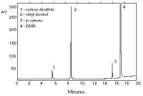 Figure 3.5.2. Chromatogram of a standard. | ||||||||||||||||||||||||||||||||||||||||||||||||||||||||||||||||||||||||||||||||||||||||||||||||||
| column: | 2.0 (H2) | ||||||||||||||||||||||||||||||||||||||||||||||||||||||||||||||||||||||||||||||||||||||||||||||||||
| split: | 258 (H2) | ||||||||||||||||||||||||||||||||||||||||||||||||||||||||||||||||||||||||||||||||||||||||||||||||||
| septum purge: | 1.8 (H2) | ||||||||||||||||||||||||||||||||||||||||||||||||||||||||||||||||||||||||||||||||||||||||||||||||||
| auxiliary: | 38 (N2) | ||||||||||||||||||||||||||||||||||||||||||||||||||||||||||||||||||||||||||||||||||||||||||||||||||
| detector air: | 375 (air) | ||||||||||||||||||||||||||||||||||||||||||||||||||||||||||||||||||||||||||||||||||||||||||||||||||
| detector H2: | 27 (H2) | ||||||||||||||||||||||||||||||||||||||||||||||||||||||||||||||||||||||||||||||||||||||||||||||||||
| miscellaneous | |||||||||||||||||||||||||||||||||||||||||||||||||||||||||||||||||||||||||||||||||||||||||||||||||||
| detector: | FID | ||||||||||||||||||||||||||||||||||||||||||||||||||||||||||||||||||||||||||||||||||||||||||||||||||
| column: | 60-m × 0.32-mm i.d. Stabilwax | ||||||||||||||||||||||||||||||||||||||||||||||||||||||||||||||||||||||||||||||||||||||||||||||||||
| injection size: | 1 µL (130:1 split) | ||||||||||||||||||||||||||||||||||||||||||||||||||||||||||||||||||||||||||||||||||||||||||||||||||
| GC retention times (min) | |||||||||||||||||||||||||||||||||||||||||||||||||||||||||||||||||||||||||||||||||||||||||||||||||||
| ethyl alcohol: | 9.0 | ||||||||||||||||||||||||||||||||||||||||||||||||||||||||||||||||||||||||||||||||||||||||||||||||||
| r-cymene: | 15.9 (internal standard) | ||||||||||||||||||||||||||||||||||||||||||||||||||||||||||||||||||||||||||||||||||||||||||||||||||
| The total GC run time was 23 min as a precaution to clear the column. | |||||||||||||||||||||||||||||||||||||||||||||||||||||||||||||||||||||||||||||||||||||||||||||||||||
3.5.3. An internal standard (ISTD) calibration method should be
used. Construct a calibration curve by plotting the ISTD corrected
detector response for each standard solution against its respective
concentration in micrograms of ethyl alcohol per sample. Determine
the
3.6. Interferences (analytical)
3.6.1. Any compound that gives an FID response and has a similar GC retention time as the analyte or the internal standard is a potential interference. Generally, chromatographic conditions can be altered to separate an interference.
3.6.2. Retention time on a single column is not proof of chemical identity. Confirmation of suspected identity should be performed by GC/mass spectrometry when necessary.
3.7. Calculations
The analyte amount per sample, micrograms of ethyl alcohol per
sample, is obtained from the calibration curve. The back tube of the
sample is analyzed primarily to determine if there was any
breakthrough from the front tube during sampling. If a significant
amount of analyte is found on the back tube (e.g., greater than 25% of
the amount found on the front tube) this fact should be reported with
sample results. If any analyte is found on the back tube it is added
to the amount on the front tube. This analyte amount is then corrected
by subtracting the total amount found in the blank. The air
concentration is obtained by using the following equations.
|
| |||||
|
|
3.8. Safety precautions (analytical)
3.8.1. Restrict the use of all chemicals to a fume hood.
3.8.2. Avoid skin contact and inhalation of all chemicals.
3.8.3. Wear safety glasses, gloves, and a lab coat at all times while working with chemicals.
4. Backup Data
4.1. Detection limit of the analytical
procedure
|
The injection size recommended in the analytical procedure (1
L, 130:1 split) was used in the determination of the detection
limit of the analytical procedure. The detection limit was 40 pg
|
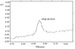 Figure 4.1. Detection limit of the analytical procedure. | |||||||||||||||
| 4.2. Detection limit of the overall
procedure
The detection limit of the overall procedure was determined
by analyzing |
| |||||||||||||||
| 4.3. Reliable quantitation limit
The reliable quantitation limit was determined by analyzing
|
| |||||||||||||||
4.4. Instrument response to the analyte
The instrument response to ethyl alcohol over the range of 0.5 to 2
times the target concentration was determined from multiple injections
of analytical standards. The response was linear with a slope of
30.6.
|
| |||
| × target concn µg/standard |
0.5× 12065 |
1.0× 23750 |
2.0× 46835 |
|
| |||
| ISTD corrected areas |
372840 381097 379231 381919 371549 377760 |
747373 721669 754169 730028 743159 745198 |
1477996 1435538 1431093 1437428 1428796 1447001 |
|
| |||
| mean | 377399.3 | 740266.0 | 1442975.3 |
|
| |||
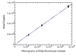
Figure 4.4.
Calibration curve for ethyl alcohol.
Thirty-six samples were collected using sampling tubes containing
Anasorb 747 (Lot 645) over 2 days (18 samples each day) from
controlled test atmospheres containing an average of 1979 ppm ethyl
alcohol. The high level of ethyl alcohol (twice the target
concentration) was used so that a sufficient number of samples to
perform a storage test could be collected in a single day's run. Each
sample was collected for 2 h at 0.05 L/min. The average relative
humidity of the controlled test atmospheres was 75% at 26°C. Six
samples (3 each day) were analyzed immediately after collection.
Fifteen samples were stored in a refrigerator at about 5°C, and 15
different samples were stored in the dark at about 23°C. Every few
days, 3 samples from each group were selected and analyzed. The
recovery of ethyl alcohol from samples stored at ambient temperature
remained above 102%.
|
| |||||||
| days of amb. storage |
% recovery (ambient) |
days of ref. storage |
% recovery (refrigerated) | ||||
|
| |||||||
| 0 | 105.0 | 105.4 | 102.4 | 0 | 102.6 | 104.4 | 100.3 |
| 3 | 104.2 | 105.4 | 103.3 | 2 | 104.3 | 105.7 | 102.9 |
| 7 | 103.4 | 101.6 | 100.7 | 6 | 102.5 | 105.5 | 102.5 |
| 10 | 104.2 | 102.9 | 103.4 | 9 | 104.8 | 103.3 | 100.4 |
| 14 | 101.3 | 102.7 | 101.6 | 13 | 106.0 | 104.9 | 103.6 |
| 16 | 104.6 | 102.3 | 101.7 | 15 | 103.4 | 106.9 | 102.9 |
|
| |||||||
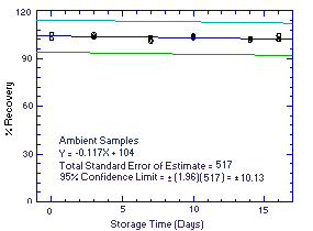
Figure 4.5.1. Ambient temperature storage test. |
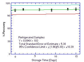
Figure 4.5.2. Refrigerated temperature storage test. |
4.6. Precision (analytical method)
The precision of the analytical procedure is defined as the pooled
coefficient of variation determined from replicate injections of
analytical standards representing 0.5, 1, and 2 times the target
concentration. The coefficients of variation are calculated from the
data in Table 4.4. The pooled coefficient of variation is
0.014.
|
| |||
| × target concn µg/sample |
0.5× 12065 |
1.0× 23750 |
2.0× 46835 |
|
| |||
| SD1 CV |
4303.5 0.0114 |
12059.5 0.0163 |
18281.0 0.0127 |
|
1 in area counts | |||
4.7. Precision (overall procedure)
The precision of the overall procedure is determined from the storage data. The determination of the standard error of estimate (SEE) for a regression line plotted through the graphed storage data allows the inclusion of storage time as one of the factors affecting overall precision. The SEE is similar to the standard deviation, except it is a measure of dispersion of data about a regression line instead of about a mean. It is determined with the following equation:
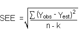
| where | n = k = k = |
total number of data points 2 for linear regression 3 for quadratic regression |
| Yobs = | observed percent recovery at a given time | |
| Yest = | estimated percent recovery from the regression line at the same given time |
An additional 5% for pump error is added to the SEE by the addition
of variances. The precision at the 95% confidence level is obtained by
multiplying the SEE (with pump error included) by 1.96 (the
| 4.8. Reproducibility data
Six samples were collected from a test atmosphere. The ethyl alcohol concentration of the test atmosphere was 1919 ppm. The relative humidity was 82% at 26°C. A draft copy of this method and the samples were submitted for analysis. The samples were analyzed after 5 days of storage at about 5°C. All of the sample results were within the precision of the overall procedure. |
| ||||||||||||||||||||
Sampler capacity was evaluated by sampling controlled test
atmospheres with
|
| |||||||
| 80% RH, 25°C | 90% RH, 25°C | 5.9% RH, 25°C | 6.1% RH, 26°C | ||||
| air vol, (L) | BT, (%) | air vol, (L) | BT, (%) | air vol, (L) | BT, (%) | air vol, (L) | BT, (%) |
|
| |||||||
| 11.9 12.3 12.8 13.2 13.5 13.7 14.3 14.7 15.2 15.6 16.1 16.5 16.7 17.4 |
0 0 0 0 0 0 0 0.1 0.8 3.8 13.6 35.1 44.0 95.9 |
5.9 8.0 9.1 10.5 12.3 13.3 14.0 14.4 14.7 15.2 15.4 15.7 16.2 17.3 |
0 0 0 0 0 0 0 0.7 2.6 11.1 19.1 29.8 48.6 72.3 |
13.7 14.7 15.7 16.7 17.2 17.4 17.9 18.4 18.9 19.2 19.5 19.7 19.9 20.2 |
0 0 0 0 0 0 0 1.1 3.6 5.9 8.4 12.7 16.0 21.3 |
7.4 8.5 9.8 14.6 15.5 16.4 16.7 17.7 17.9 18.1 18.6 18.9 19.1 19.6 |
0 0 0 0 0 0 0 0 1.3 1.5 3.7 6.5 8.6 16.8 |
|
| |||||||
| RH = relative humidity | BT = breakthrough | ||||||
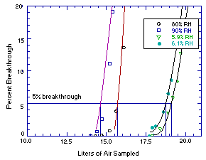
Figure 4.9. Sampler
capacity tests.
4.10. Desorption efficiency and stability of
desorbed samples
| 4.10.1. Desorption efficiency
The desorption efficiency of ethyl alcohol from Anasorb 747
was determined by liquid spiking |
| ||||||||||||||||||||||||||||
4.10.2. Stability of desorbed samples
The stability of desorbed samples was verified by reanalyzing the
1.0 times target concentration samples following the original
analysis. Samples are considered stable if the average of the
percent difference between the initial and the reanalyzed samples is
less than ±5% [average(% initial-% reanalyzed)<5%]. The samples
were resealed immediately after the original analysis and fresh
standards were used in the reanalysis. Both the original desorbed
samples
|
| ||||||||||||||||||||||||||||||
4.10.3. Desorption efficiency of other analytes
The desorption efficiencies of other analytes from Anasorb 747
was determined by liquid spiking
|
| ||||||||||||||||||||||||||||||||||||||||||||||||||||||||||||||||||||||
| | |||||||||||||||||||||||||||||||||||||||||||||||||||||||||||||||||||||||
|
| ||||||||||||||||||||||||||||||||||||||||||||||||||||||||||||||||||||||
|
| ||||
| × target concn µg/sample |
0.1× 122 |
0.5× 630 |
1.0× 1259 |
2.0× 2518 |
|
| ||||
| DE, % | 103.3 102.2 101.8 99.6 102.4 102.8 |
97.3 102.8 102.1 101.9 103.5 102.6 |
102.6 98.6 99.9 91.2 102.1 99.5 |
98.0 97.5 100.2 99.2 100.8 95.6 |
|
| ||||
| mean | 102.0 | 101.7 | 99.0 | 98.6 |
|
average DE over the studied range was 100.3% | ||||
5. References
5.1. NIOSH Manual of Analytical Methods,
3rd. ed; Eller, P.M., Ed.; U.S. Department of Health and Human
Services, Public Health Service, Centers for Disease Control, National
Institute for Occupational Safety and Health, Division of Physical
Sciences and Engineering: Cincinnati, DHHS (NIOSH) Publication No.
5.2. Hendricks, W. "OSHA Method No. 91, Methyl
Alcohol"; OSHA Salt Lake Technical Center, unpublished, Salt Lake
City, UT
5.3. Harper, M. Technical Information Sheet:
5.4. Documentation of the Threshold Limit Values and Biological Exposure Indices, 5th. ed.; American Conference of Governmental Industrial Hygienists, Inc.: Cincinnati, 1986; p 242.2.
5.5. Code of Federal Regulations, Title
29, 1910.1000, Table
5.6. Kirk-Othmer Encyclopedia of Chemical
Technology, 3rd ed.; Grayson, M. Ed.; John Wiley & Sons: New
York, 1980, Vol. 9; pp
5.7. OSHA Computerized Information System
Database, Occupational Health Services, Inc. (OHS) MSDS File; Ethyl
Alcohol; Revision Date: 06/23/92; OSHA SLTC, Salt Lake City, UT
5.8. IARC Monographs on the Evaluation of Carcinogenic Ricks to Humans, Alcohol Drinking; Volume 44; International Agency for Research on Cancer, Secretariat of the World Health Organization: UK, 1988; ISBN 92 832 1244 4.
5.9. Hawley's Condensed Chemical
Dictionary; 11th ed.; Revised by Sax, I.N. and Lewis, R.J.; Van
Nostrand and Reinhold: New York, 1987; pp
5.10. Hawley's Condensed Chemical Dictionary; 11th ed.; Revised by Sax, I.N. and Lewis, R.J.; Van Nostrand and Reinhold: New York, 1987; p 31.
5.11. Anderson, E.V. Chem. Eng. News
1992, 70(44),