![]()
| Method number: | 112 |
| Matrix: | Air |
| Target concentration: OSHA PEL: ACGIH TLV: |
25 ppm (90.5 mg/m3) TWA, (skin) 25 ppm (90.5 mg/m3) TWA, (skin) 10 ppm (36.2 mg/m3) (skin) |
| Procedure: | Samples are collected by drawing known volumes of air through sampling tubes containing 600 mg of Chromosorb 106 in the front section and 300 mg in the back section. Keep the samples in a refrigerator to help minimize analyte migration. Samples are desorbed with toluene and analyzed by GC using an electron capture detector. |
| Recommended air volume and sampling rate: |
6 L at 50 mL/min (120 min) |
| Reliable quantitation limit: | 22 ppb (80 µg/m3) |
| Standard error of estimate at the target concentration: |
7.9% |
| Status of method: | Evaluated method. This method has been subjected to the established evaluation procedures of the Organic Methods Evaluation Branch. |
| Date: September 1998 | Chemist: Yihlin Chan |
Organic Methods Evaluation Branch
OSHA Salt Lake
Technical Center
Salt Lake City, UT 84115-1802
1. General Discussion
- 1.1 Background
- 1.1.1 History
For monitoring occupational exposure to chloroprene, NIOSH specifies sampling with coconut shell charcoal tubes, desorption with carbon disulfide, and analysis by GC with a flame ionization detector (FID) (Ref. 5.1). Work at OSHA SLTC, however, has shown that the coconut shell charcoal tube does not retain chloroprene well (Ref. 5.2). Also, the method is not very sensitive. The present work was undertaken to develop a sampling and analytical method that is more sensitive.
Chloroprene auto-oxidizes easily, polymerizes spontaneously at
room temperature, and forms cyclic dimers on prolonged standing even
in the presence of polymerization inhibitors (Ref.
5.3). Attempts were made to convert chloroprene to a stable
derivative. The reagents investigated included bromine, hydrogen
bromide, tetracyanoethylene, and
In 1987, a Chinese scientist reported a method of determining the
concentration of chloroprene in air down to 0.01
mg/m3 (3 ppb) (Ref.
5.4). He sampled with tubes containing Chromosorb 101 and
thermally desorbed the analyte directly into a GC column. Because
the sample is not diluted with solvents, sensitivity is greatly
enhanced -
Chromosorb 106 was selected as the sampling media for its high
surface area (700 to 800 m2/g versus less
than 50 m2/g for Chromosorb 101). The
selection was also based on the consideration that the method may be
adapted to thermal desorption in the future. The sensitivity was
increased
There was concern for the purity of chloroprene used to prepare
analytical standards because chloroprene is unstable. NIOSH used
freshly distilled chloroprene in their method. (Ref.
5.1). We recommend the same. There are two commercially
available sources of chloroprene: Chem Service (45% in xylene) and
Alfa/Aeser (50% in xylene). When materials from these two suppliers
were compared with freshly distilled chloroprene, their nominal
concentrations were within experimental error. They were found to be
stable when stored in a freezer
1.1.2 Toxic effects (This section is for information only and should not be taken as the basis of OSHA policy.)
Chloroprene is much more toxic to rodents than butadiene or
isoprene. Toxic effects in humans from acute,
1.1.3 Workplace exposure
Most chloroprene is polymerized to make polychloroprene
(neoprene), a synthetic rubber used in wire and cable covers,
gaskets, automotive parts, adhesives, caulks,
1.1.4 Physical properties and other descriptive information (Ref. 5.2)
| CAS no.: | 126-99-8 |
| synonyms: | |
| formula: | C4H5Cl |
| formula weight: | 88.54 |
| appearance: | clear liquid |
| boiling point: | 59.4 °C |
| melting point: | -128 to -132 °C |
| density: | 0.9585 g/mL at 20 °C 0.9591 g/mL at -12 °C 0.9148 g/mL (50% in xylene, at -12 °C) 0.9106 g/mL (calculated for 45% in xylene, at -12 °C) |
| flash point: | -20 °C (ASTM open cup) |
| solubility: | slightly soluble in water (<1%) and miscible with most organic solvents |
| vapor pressure (p): | log10p = 6.652 - 1545/T (T in K, p in kPa) |
| reactivity: | readily forms dimers and oxidizes at room temperature |
| structure: |  |
The analyte air concentrations throughout this method are based on the recommended sampling and analytical parameters. Air concentrations listed in ppm are referenced to 25 °C and 101.3 kPa (760 mmHg).
1.2 Limit defining parameters
- 1.2.1 Detection limit of the analytical procedure
The detection limit of the analytical procedure is 2.4 pg. This is the amount of analyte that will give a response that is significantly different from the background response of reagent blank. (Sections 4.1 and 4.2)
1.2.2 Detection limit of the overall procedure
The detection limit of the overall procedure is 0.14 µg per sample (6.6 ppb, 24 µg/m3). This is the amount of analyte spiked on the sampler that will give a response that is significantly different from the background response of a sampler blank. (Sections 4.1 and 4.3)
1.2.3 Reliable quantitation limit
The reliable quantitation limit is 0.48 µg per sample (22 ppb, 80 µg/m3). This is the amount of analyte spiked on a sampler that will give a signal that is considered the lower limit for precise quantitative measurements. (Section 4.4)
1.2.4 Precision (analytical procedure)
The precision of the analytical procedure, measured as the pooled relative standard deviation over a concentration range equivalent to 0.5 to 2 times the target concentration, is 0.32%. (Section 4.5)
1.2.5 Precision (overall procedure)
The precision of the overall procedure at the 95% confidence
level for the ambient
1.2.6 Recovery
The recovery of chloroprene from samples used in a
1.2.7 Reproducibility
Six samples, collected from a controlled test atmosphere of chloroprene, with a draft copy of this procedure, were submitted for analysis by an SLTC Service Branch. The samples were analyzed after 2 days of storage at 5 °C. No individual sample result deviated from its theoretical value by more than the precision reported in Section 1.2.5. (Section 4.8)
2. Sampling Procedure
- 2.1 Apparatus
- 2.1.1 A personal sampling pump calibrated to ±5% of the
recommended flow rate with the sampling device attached.
2.1.2 Glass sampling tubes (150 mm × 10 mm o.d.) packed with two
sections of Chromosorb 106. The front section contains 600 mg and
the back section contains 300 mg. The sections are held in place
with glass wool plugs. For this evaluation, commercially prepared
sampling tubes were purchased from SKC, Inc. (Catalog no.
2.2 Reagents
None required.
2.3 Technique
- 2.3.1 Immediately before sampling, break off the ends of the
sampling tube. All tubes should be from the same lot.
2.3.2 Attach the sampling tube to the sampling pump with flexible tubing.
2.3.3 Air should not pass through any hose or tubing before entering the sampling tube.
2.3.4 Cap both ends after sampling. Wrap each sample with a Form
2.3.5 Record the air volume for each sample.
2.3.6 Submit at least one blank with each set of samples. Blanks should be handled in the same manner as samples, except no air is drawn through them.
2.3.7 List any compounds that could be considered potential interferences.
2.4 Sampler capacity
The capacity of the front section of the SKC
2.5 Desorption efficiency
- 2.5.1 The average desorption efficiency for chloroprene from
Chromosorb 106 over the range of 0.5 to 2.0 times the target
concentration was 101.9%. (Section
4.10.1)
2.5.2 The desorption efficiencies at 0.05, 0.1, and 0.2 times the target concentration were found to be 100.8%, 101.0%, and 101.1%, respectively. (Section 4.10.1)
2.5.3 Desorbed samples remain stable for at least 24 h. (Section 4.10.2)
2.6 Recommended air volume and sampling rate
- 2.6.1 The recommended air volume is 6 L at 50 mL/min.
2.6.2 For
2.6.3 When
2.7 Interferences (sampling)
There is no known interference for sampling.
2.8 Safety precautions (sampling)
- 2.8.1 The sampling equipment should be attached to the worker in
such a manner that it will not interfere with work performance or
safety.
2.8.2 All safety practices that apply to the work area being sampled should be followed.
3. Analytical Procedure
- 3.1 Apparatus
- 3.1.1 A GC equipped with an electron capture detector (ECD). An
HP 5890 equipped with an ECD and an autosampler were used in this
evaluation.
3.1.2 A capillary column capable of separating chloroprene and
the internal standard (trichloroethylene) from any interferences. An
3.1.3 An electronic integrator or other suitable means of measuring detector response. The Millennium Chromatography Manager System (Waters) was used in this evaluation.
3.1.4 Glass vials, 4-mL and 2-mL, with
3.1.5 A dispenser capable of delivering 2.00 mL of desorbing solvent.
3.2 Reagents
- 3.2.1 Chloroprene. Chloroprene, 50% in xylene, was obtained from
Alfa/Aesar. Chloroprene, 45% in xylene, was obtained from Chem
Service. They were stored in a freezer at
3.2.2 Toluene. Toluene, b&j high purity solvent grade, was obtained from Baxter.
3.2.3 Trichloroethylene. Trichloroethylene, 99.5+%, was obtained from Aldrich Chemical.
3.2.4 Desorbing solvent. Dilute 5.0 µL of trichloroethylene with 1000 mL of toluene.
3.3 Standard preparation
- 3.3.1 Distill chloroprene from its xylene solution (Section
4.12). Determine the concentration (w/w) of the 50% chloroprene
in xylene using the freshly distilled chloroprene as reference. The
50% chloroprene solution should be stored in a freezer and its
concentration checked within a month of analysis. Determine the
density of the solution if it is measured by volume instead of
weight. Alternatively, use the reference standard of chloroprene
supplied by Chem Service whose concentration is guaranteed to be
within ±0.5% prior to the expiration date.
3.3.2 Prepare analytical standards by diluting the reference
standards with the desorbing solvent. Prepare fresh analytical
standards daily. A
3.4 Sample preparation
- 3.4.1 Transfer the sorbent of the front and the back section to
separate
3.4.2 Add 2.00 mL of the desorbing solvent to each vial.
3.4.3 Cap the vials and shake them on a shaker for 30 min.
3.4.4. Pour the solution into a
3.5 Analysis
- 3.5.1 GC conditions
| column: | Rtx-1 (60 m × 0.32-mm i.d., 1.0-µm df) |
| oven temperature: | 70 °C for 8 min, 30/min to 250 °C, hold for 5 min at 250 °C. |
| inlet temperature: | 250 °C |
| detector temperature: | 250 °C |
| injection size: | 1.0 µL |
| retention time: | 4.8 min (chloroprene) 7.0 min (trichloroethylene) |
| carrier gas (H2): | 1.8 mL/min |
| make-up gas (N2): | 45.3 mL/min |
| split vent: | 22.7 mL/min |
| split ratio: | 13.7 : 1 |
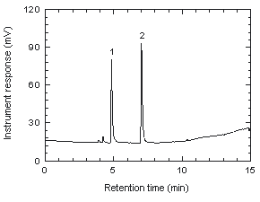
Figure 3.5.1. Chromatogram at target concentration.
1 = chloroprene, 2 = internal standard.
| 3.5.2 An internal standard calibration method is used. A
calibration curve can be constructed by plotting concentration
of the analyte versus |
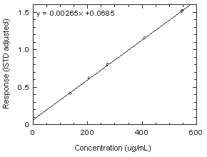 Figure 3.5.2. Calibration curve of chloroprene from the data of Table 4.5. |
3.6 Interferences (analytical)
- 3.6.1 Any compound that produces an ECD response and has a
similar retention time as the analyte or the internal standard is a
potential interference. If any potential interferences are reported,
they should be considered before samples are desorbed. Generally,
chromatographic conditions can be altered to separate an
interference from the analyte.
3.6.2 Any compound that affects the ECD response is a potential interference. The oven temperature program in Section 3.5.1 should be followed to remove any late eluting peak after each injection.
3.6.3 When necessary, the identity or the purity of an analyte peak may be confirmed with additional analytical data (Section 4.11).
3.7 Calculations
The amount (in micrograms) of chloroprene per milliliter is obtained from the calibration curve. This amount is corrected by subtracting the amount (if any) found in the blank. The air concentration is calculated using the following formula.
| mg/m3 = | (liters of air sampled) × (desorption efficiency) |
| ppm = (mg/m3) × | MW |
| where: | desorption volume = 2.00 mL desorption efficiency = 1.05 MW = 88.54 |
3.8 Safety precautions (analytical)
- 3.8.1 Follow the rules set down in your Chemical Hygiene Plan.
3.8.2 Wear appropriate gloves. Avoid skin contact and inhalation of all chemicals.
3.8.3 Wear safety glasses and a lab coat at all times while in the lab area.
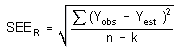
- 4.1 Determination of detection limits
Detection limits (DL), in general, are defined as the amount (or concentration) of analyte that gives a response (YDL) that is significantly different (three standard deviations (SDBR)) from the background response (YBR).
YDL - YBR = 3(SDBR)
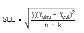
The direct measurement of YBR and SDBR in chromatographic methods is typically inconvenient and difficult because YBR is usually extremely low. Estimates of these parameters can be made with data obtained from the analysis of a series of analytical standards or samples whose responses are in the vicinity of the background response. The regression curve obtained for a plot of instrument response versus concentration of analyte will usually be linear. Assuming SDBR and the precision of data about the curve are similar, the standard error of estimate (SEE) for the regression curve can be substituted for SDBR in the above equation. The following calculations derive a formula for DL:
| Yobs = | observed response |
| Yest = | estimated response from regression curve |
| n = | total no. of data points |
| k = | 2 for a linear regression curve |
At point YDL on the regression curve
- YDL = A(DL) +
YBR A
= analytical sensitivity (slope)
therefore
| DL = | A |
Substituting 3(SEE) + YBR for YDL gives
| DL = | A |
4.2 Detection limit of the analytical procedure (DLAP)
The DLAP is measured as the mass of analyte actually introduced
into the chromatographic column. Ten analytical standards of
chloroprene whose concentrations were equally spaced from 0 to 0.532
µg/mL were prepared. The standard containing 0.532 µg/mL
represented approximately 10 times the baseline noise. These solutions
were analyzed with the recommended analytical parameters
|
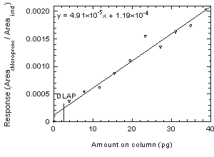 Figure 4.2. Plot of data to determine the DLAP. | |||||||||||||||
| * response = (peak area chloroprene)/(peak area ISTD) | ||||||||||||||||
4.3 Detection limit of the overall procedure (DLOP)
The DLOP is measured as mass per sample and expressed as equivalent air concentration, based on the recommended sampling parameters. Ten samplers were spiked with chloroprene ranging from 0 to 1.06 µg. The latter amount, when spiked on a sampler, would produce a peak approximately 10 times the baseline noise for a sample blank. These samples were analyzed with the recommended analytical parameters, and the data obtained used to calculate the required parameters (A and SEE) for the calculation of the DLOP. Values of 1.94 × 10⁻³ and 9.32 × 10⁻⁵ were obtained for A and SEE respectively. DLOP was calculated to be 0.14 µg/sample (24 µg/m3 or 6.6 ppb).
|
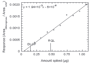 Figure 4.3. Plot of data to obtain DLOP and RQL. | |||||||||||
| * response = (peak area chloroprene)/(peak area ISTD) | ||||||||||||
4.4 Reliable quantitation limit
| The RQL is considered the lower limit for precise
quantitative measurements. It is determined from the regression
line data obtained for the calculation of the DLOP (Section
4.3), providing at least 75% of the analyte is recovered.
The RQL is defined as the amount of analyte that gives a
response (YRQL) such that
YRQL - YBR = 10(SDBR) therefore
|
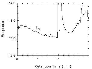 Figure 4.4. Chromatogram near RQL. 1 = chloroprene, 2 = trichloroethylene, 3 = unknown impurity. |
RQL = 0.48 µg per sample (80 µg/m3 or 22 ppb)
Recovery at this level is 88%.
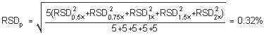
4.5 Precision (analytical method)
The precision of the analytical procedure is defined as the pooled relative standard deviation (RSDP). Relative standard deviations were determined from six replicate injections of analytical standards at 0.5, 0.75, 1, 1.5, and 2 times the target concentration. After assuring that the RSDs satisfy the Cochran test for homogeneity at the 95% confidence level, RSDp was calculated.
The Cochran test for homogeneity requires the calculation of the g statistics according to the following formula:
| g = | largest RSD2
|
= 0.4758 |
The critical value of the g statistic, at the 95% confidence level, for five variances, each associated with six observations, is 0.5065. Because the g statistic obtained (0.4758) does not exceed this value, the RSDs within each level can be considered equal and they can be pooled (RSDP) to give an estimated RSD for the concentration range studied.
4.6 Precision (overall procedure)
The precision of the overall procedure is determined from the storage data in Section 4.7. The determination of the standard error of estimate (SEER) for a regression line plotted through the graphed storage data allows the inclusion of storage time as one of the factors affecting overall precision. The SEER is similar to the standard deviation, except it is a measure of dispersion of data about a regression line instead of about a mean. It is determined with the following equation:
| n = k = k = |
total no. of data points 2 for linear regression 3 for quadratic regression |
| Yobs = | observed % recovery at a given time |
| Yest = | estimated % recovery from the regression line at the same given time |
An additional 5% for pump error (SP) is added to the SEER by the addition of variances to obtain the total standard error of estimate.
![]()
The precision at the 95% confidence level is obtained by
multiplying the standard error of estimate (with pump error included)
by 1.96 (the
Storage samples were prepared by drawing a controlled test
atmosphere (80% relative humidity and 22°C) through samplers at 50
mL/min for 120 min. The concentration of chloroprene was approximately
at the target concentration.
|
| |||||||
| time (days) |
percent recovery (ambient) |
percent
recovery (refrigerated) | |||||
|
| |||||||
| 0 | lost | 100.7 | 99.3 | lost | 100.7 | 99.3 | |
| 0 | 100.1 | 99.9 | lost | 100.1 | 99.9 | lost | |
| 0 | 100.4 | 99.3 | 100.3 | 100.4 | 99.3 | 100.3 | |
| 3 | 101.3 | 103.8 | 100.1 | 102.2 | lost | 102.9 | |
| 4 | 96.8 | 99.5 | 99.4 | ||||
| 6 | 97.5 | 97.0 | 74.6* | 100.3 | 100.9 | 98.6 | |
| 7 | 95.1 | 96.8 | 101.0 | ||||
| 9 | 97.5 | 89.9 | 95.5 | 100.6 | 53.5* | 101.9 | |
| 11 | 83.4 | 96.8 | 89.2 | ||||
| 13 | 87.4 | 83.7 | 81.1 | 92.0 | 93.1 | 92.2 | |
| 13 | 100.1 | 100.8 | 95.7 | ||||
| 15 | 105.1 | 102.2 | 104.0 | 99.7 | 104.1 | 99.1 | |
| 15 | 99.0 | 96.3 | 98.0 | ||||
|
Lost = tube broken or tubing came off during sampling *outlier, not used | |||||||
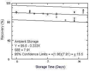 Figure 4.7.1. Ambient storage test for chloroprene. |
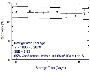 Figure 4.7.2. Refrigerated storage test for chloroprene. |
Reproducibility samples were prepared by collecting them from a controlled test atmosphere similar to that used in the storage test. The samples were submitted to an SLTC Service Branch for analysis. The samples were analyzed after being stored for 2 days at 5°C. No sample result had a deviation greater than the precision of the overall procedure determined in Section 4.7.
|
| |||
| ppm expected | ppm found | percent found | percent deviation |
|
| |||
| 26.7 | 25.6 | 95.9 | -4.1 |
| 26.7 | 26.0 | 97.4 | -2.6 |
| 26.7 | 26.0 | 97.4 | -2.6 |
| 26.7 | 25.4 | 95.1 | -4.9 |
| 26.7 | 25.6 | 95.9 | -4.1 |
| 26.7 | 26.4 | 98.9 | -1.1 |
|
| |||
The capacity of the front section of a Chromosorb 106 tube (SKC
|
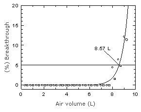 Figure
4.9. Breakthrough curve for chloroprene on Chromosorb 106 at two
times the target concentration. Figure
4.9. Breakthrough curve for chloroprene on Chromosorb 106 at two
times the target concentration. | |||||||||||||||||||||||||||||
4.10 Desorption efficiency and stability of desorbed samples
- 4.10.1 Desorption efficiency
The desorption efficiencies (DE) test samples were prepared by
|
| ||||||
| × target concn (µg/sample) |
0.05 × 26.6 |
0.1 × 53.2 |
0.2 × 10⁶ |
0.5 × 266 |
1.0 × 532 |
2.0 × 1063 |
|
| ||||||
| DE (%) | 101.0 | 100.5 | 100.8 | 101.3 | 101.0 | 102.4 |
| 101.2 | 100.5 | 101.4 | 100.9 | 103.5 | 102.7 | |
| 100.8 | 100.3 | 101.8 | 101.1 | 101.8 | 102.5 | |
| 100.7 | 101.4 | 101.3 | 101.1 | 102.0 | 102.8 | |
| 100.3 | 101.7 | 101.2 | 100.9 | 102.2 | 103.0 | |
| 100.8 | 101.5 | 99.9 | 100.5 | 102.0 | 103.0 | |
| Average | 100.8 | 101.0 | 101.1 | 101.0 | 102.1 | 102.7 |
|
| ||||||
4.10.2 Stability of desorbed samples
The stability of the desorbed samples was investigated by
|
| |||||
| punctured septa replaced | punctured septa retained | ||||
|
| |||||
| initial DE (%) |
DE after one day (%) |
difference | initial DE (%) |
DE after one day (%) |
difference |
|
| |||||
| 101.0 | 99.0 | -2.0 | 102.0 | 98.2 | -3.8 |
| 103.5 | 99.2 | -4.3 | 102.2 | 98.5 | -3.7 |
| 101.8 | 99.9 | -1.9 | 102.0 | 98.4 | -3.5 |
| average | average | ||||
| 102.1 | 99.4 | -2.7 | 102.1 | 98.4 | -3.7 |
|
| |||||
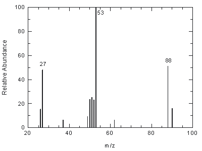
Chloroprene may be confirmed by GC/MS using GC conditions similar to those in Section 3.5.1.
Figure
4.11. Mass spectrum of 2-chloro-1,3-butadiene.
4.12 Distillation of chloroprene
Chloroprene was distilled at atmospheric pressure (650 mmHg). The
cut boiling between 62°C and 66°C was collected. Freshly distilled
chloroprene was stored at
5. References
- 5.1. NIOSH Manual of Analytical Methods,
Fourth Edition, U.S. Department of Health and Human Services, Center
for Disease Control, National Institute for Occupational Safety and
Health, Cincinnati, OH, DHHS (NIOSH) Publication No.
5.2. Eide, M. OSHA SLTC, Salt Lake City, UT, A
Study of the Detection
5.3. Johnson, P. R. in Kirk-Othmer
Encyclopedia of Chemical Technology, 3rd edition,
1982, Vol. 5,
5.4. Wang, P. Chromatographical Determination of
Traces of
5.5. IARC Monographs on the Evaluation of the
Carcinogenic Risk of Chemicals to Humans, International Agency for
Research on Cancer, Lyon, 1979, 19,
5.6. Documentation of the Threshold Limit Values and Biological Exposure Indices, 6th Edition, 1991, American Conference of Governmental Industrial Hygienist, Cincinnati, OH.
5.7. NIOSH criteria for a recommended standard
... occupational exposure to Chloroprene, U.S. Department of
Health, Education, and Welfare, Center for Disease Control, National
Institute for Occupational Safety and Health, Cincinnati, OH DHEW
(NIOSH) Publication No.